Analyze query profile

This topic describes how to check the query profile. A query profile records the execution information of all worker nodes involved in a query. Query profiles help you quickly identify the bottlenecks that affect the query performance of your StarRocks cluster.

Enable query profile

For StarRocks versions earlier than v2.5, you can enable query profile by setting the variable is_report_success to true:

set is_report_success = true;

For StarRocks v2.5 or later versions, you can enable query profile by setting the variable enable_profile to true:

set enable_profile = true;

Access query profiles

Follow these steps to access your query profiles:

1. Enter http://<fe_ip>:<fe_http_port> in your browser.
2. On the page this is displayed, click queries on the top navigation pane.
3. In the Finished Queries list, choose the query you want to check and click the link in the Profile column.

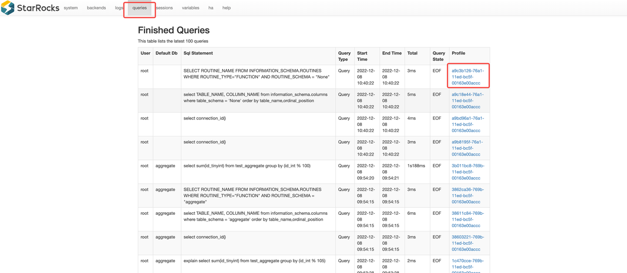
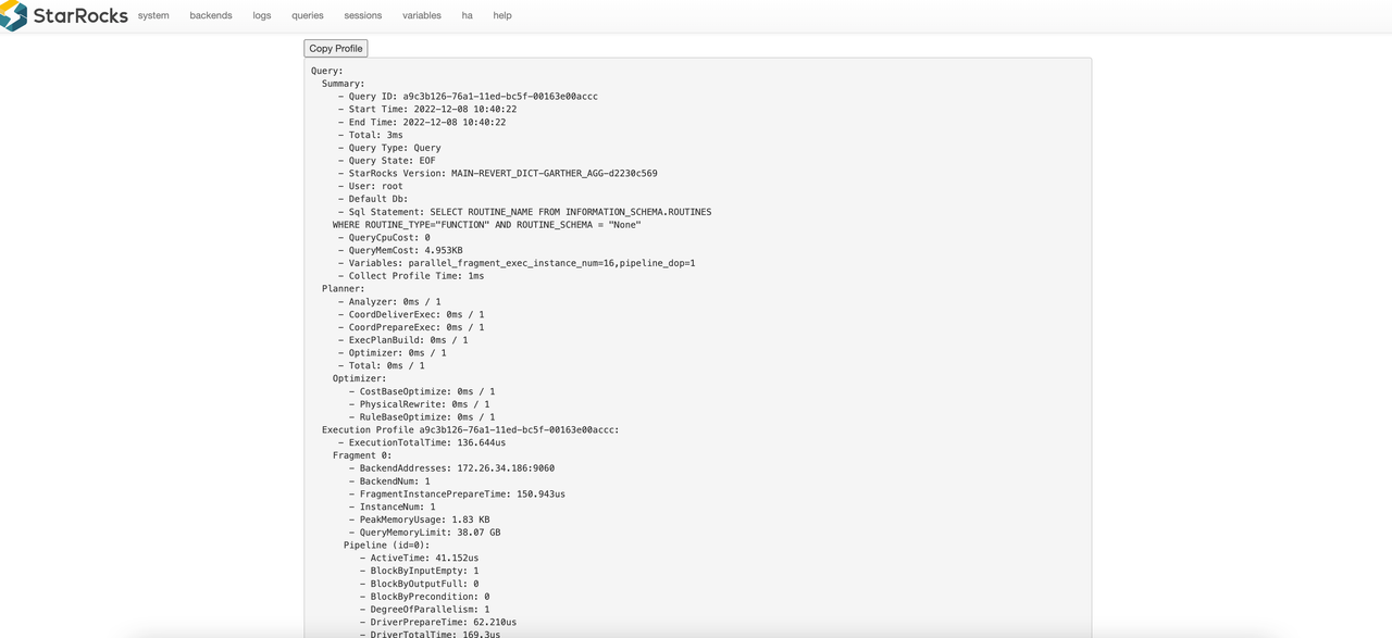
The browser redirects you to a new page that contains the corresponding query profile.

Interpret a query profile

Structure of a query profile

Following is an example query profile:

Query:
  Summary:
  Planner:
  Execution Profile 7de16a85-761c-11ed-917d-00163e14d435:
    Fragment 0:
      Pipeline (id=2):
        EXCHANGE_SINK (plan_node_id=18):
        LOCAL_MERGE_SOURCE (plan_node_id=17):
      Pipeline (id=1):
        LOCAL_SORT_SINK (plan_node_id=17):
        AGGREGATE_BLOCKING_SOURCE (plan_node_id=16):
      Pipeline (id=0):
        AGGREGATE_BLOCKING_SINK (plan_node_id=16):
        EXCHANGE_SOURCE (plan_node_id=15):
    Fragment 1:
       ...
    Fragment 2:
       ...

A query profile consists of three sections:

• Fragment: the execution tree. One query can be divided into one or more fragments.
• Pipeline: the execution chain. An execution chain does not have branches. A fragment can be split into several pipelines.
• Operator: A pipeline consists of a number of operators.

A fragment consists of several pipelines.

Key metrics

A query profile encompasses a mass of metrics that show the details of the query execution. In most cases, you only need to observe the execution time of the operators and the size of the data that they processed. After finding the bottlenecks, you can solve them accordingly.

Summary

Metric	Description
Total	Total time consumed by the query, including the time spent in planning, executing, and profiling.
QueryCpuCost	Total CPU time cost of the query. CPU time costs are aggregated for concurrent processes. As a result, the value of this metric may be greater than the actual execution time of the query.
QueryMemCost	Total memory cost of the query.

Universal metrics for operators

Metric	Description
OperatorTotalTime	Total CPU time cost of the operator.
PushRowNum	Total row count of the data that the operator pushed.
PullRowNum	Total row count of the data that the operator pulled.

Scan operator

Metric	Description
Table	Table name.
ScanTime	Total scan time. Scans are performed in the asynchronous I/O thread pool.
TabletCount	Number of tablets.
PushdownPredicates	Number of the predicates that were pushed down.
BytesRead	Size of the data read by StarRocks.
CompressedBytesRead	Size of the compressed data read by StarRocks.
IOTime	Total I/O time.
BitmapIndexFilterRows	Row count of the data that were filtered out by Bitmap index.
BloomFilterFilterRows	Row count of the data that were filtered out by Bloomfilter.
SegmentRuntimeZoneMapFilterRows	Row count of the data that were filtered out by runtime Zone Map.
SegmentZoneMapFilterRows	Row count of the data that were filtered out by Zone Map.
ShortKeyFilterRows	Row count of the data that were filtered out by Short Key.
ZoneMapIndexFilterRows	Row count of the data that were filtered out by Zone Map index.

Exchange operator

Metric	Description
PartType	Data distribution type. Valid values: UNPARTITIONED, RANDOM, HASH_PARTITIONED, and BUCKET_SHUFFLE_HASH_PARTITIONED.
BytesSent	Size of the data that were sent.
OverallThroughput	Overall throughput.
NetworkTime	Data package transmission time (excluding the time of post-receiving processing). See FAQ below for more about how this metric is calculated and how it can hit an exception.
WaitTime	Time to wait because the queue at the sender side is full.

Aggregate operator

Metric	Description
GroupingKeys	Name of the grouping keys (GROUP BY columns).
AggregateFunctions	Aggregate functions.
AggComputeTime	Compute time consumed by aggregate functions.
ExprComputeTime	Compute time consumed by the expression.
HashTableSize	Size of the hash table.

Join operator

Metric	Description
JoinPredicates	Predicates of the JOIN operation.
JoinType	The JOIN type.
BuildBuckets	Bucket number of the hash table.
BuildHashTableTime	Time used to build the hash table.
ProbeConjunctEvaluateTime	Time consumed by Probe Conjunct.
SearchHashTableTimer	Time used to search the hash table.

Window Function operator

Metric	Description
ComputeTime	Compute time consumed by the window function.
PartitionKeys	Name of the partitioning keys (PARTITION BY columns).
AggregateFunctions	Aggregate functions.

Sort operator

Metric	Description
SortKeys	Name of the sort keys (ORDER BY columns).
SortType	Result sorting type: to list all results, or to list top n results.

TableFunction operator

Metric	Description
TableFunctionExecTime	Compute time consumed by the table function.
TableFunctionExecCount	Number of times the table function is executed.

Project operator

Metric	Description
ExprComputeTime	Compute time consumed by the expression.
CommonSubExprComputeTime	Compute time consumed by the common sub-expression.

LocalExchange operator

metric	Description
Type	Local Exchange type. Valid values: Passthrough, Partition, and Broadcast.
ShuffleNum	Number of shuffles. This metric is valid only when Type is Partition.

Time consumed by operators

• For the OlapScan and ConnectorScan operators, their time consumption is equivalent to OperatorTotalTime + ScanTime. Because the Scan operators perform I/O operations in the asynchronous I/O thread pool, ScanTime represents asynchronous I/O time.
• The time consumption of the Exchange operator is equivalent to OperatorTotalTime + NetworkTime. Because the Exchange operator sends and receives data packages in the bRPC thread pool, NetworkTime represents the time consumed by network transmission.
• For all other operators, their time cost is OperatorTotalTime.

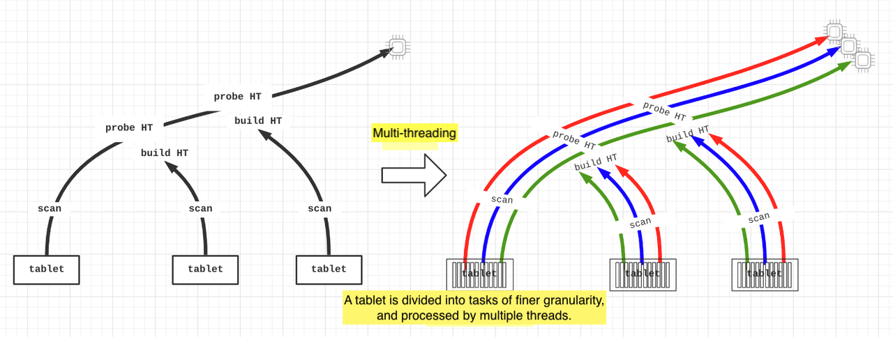
Metric merging and MIN/MAX

Pipeline engine is a parallel computing engine. Each fragment is distributed to multiple machines for parallel processing, and pipelines on each machine are executed in parallel as multiple concurrent instances. Therefore, while profiling, StarRocks merges same metrics, and records the minimum and maximum values of each metric among all the concurrent instances.

Different merging strategies are adopted for different types of metrics:

• Time metrics are averages. For example:
  • OperatorTotalTime represents the average time cost of all the concurrent instances.
  • __MAX_OF_OperatorTotalTime is the maximum time cost among all the concurrent instances.
  • __MIN_OF_OperatorTotalTime is the minimum time cost among all the concurrent instances.

             - OperatorTotalTime: 2.192us
               - __MAX_OF_OperatorTotalTime: 2.502us
               - __MIN_OF_OperatorTotalTime: 1.882us

• Non-time metrics are totaled. For example:

  • PullChunkNum represents the total number of all concurrent instances.
  • __MAX_OF_PullChunkNum is the maximum value among all the concurrent instances.
  • __MIN_OF_PullChunkNum is the minimum value among all the concurrent instances.

                 - PullChunkNum: 146.66K (146660)
                   - __MAX_OF_PullChunkNum: 24.45K (24450)
                   - __MIN_OF_PullChunkNum: 24.435K (24435)

• Some special metrics, which do not have minimum and maximum values, have identical values among all the concurrent instances (for example, DegreeOfParallelism).

Sharp difference between MIN and MAX

Usually, a noticeable difference between MIN and MAX values indicates the data is skewed. It possibly happens during aggregate or JOIN operations.

             - OperatorTotalTime: 2m48s
               - __MAX_OF_OperatorTotalTime: 10m30s
               - __MIN_OF_OperatorTotalTime: 279.170us

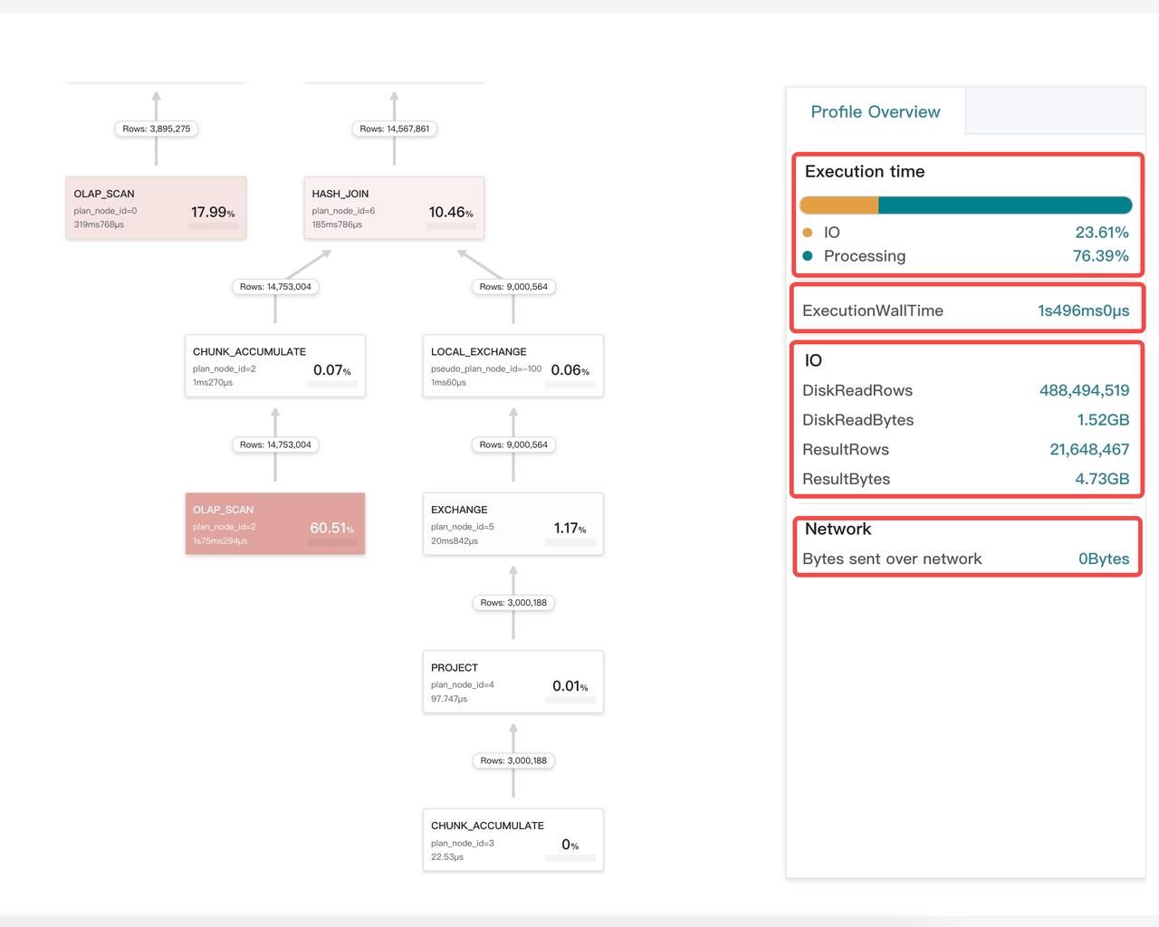
Visualize a query profile

If you are a user of StarRocks Enterprise Edition, you can visualize your query profiles via StarRocks Manager.

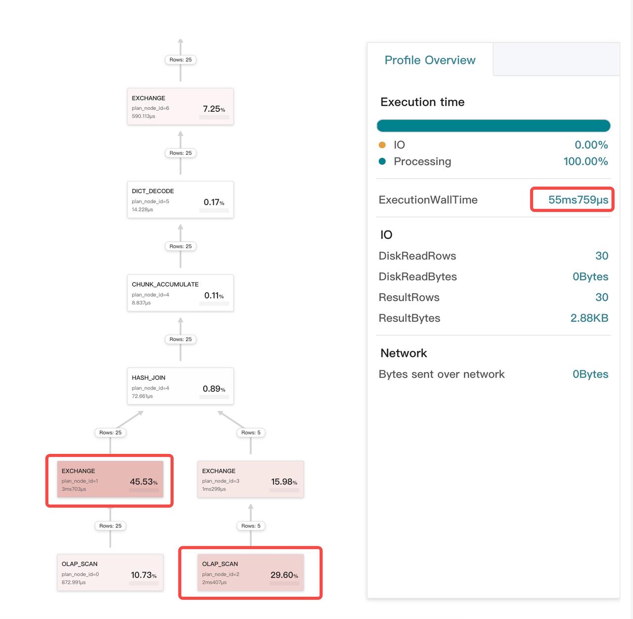
The Profile Overview page displays some summary metrics, including the total execution time ExecutionWallTime, I/O metrics, network transmission size, and the proportion of CPU and I/O time.

By clicking the card of an operator (a node), you can view its detailed information in the right pane of the page. There are three tabs:

• Node: core metrics of this operator.
• Node Detail: all metrics of this operator.
• Pipeline: metrics of the pipeline to which the operator belongs. You do not need to pay much attention to this tab because it is related only to scheduling.

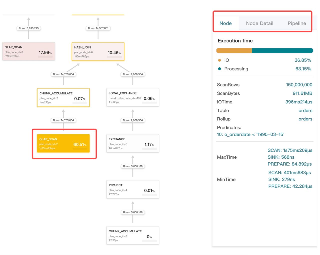
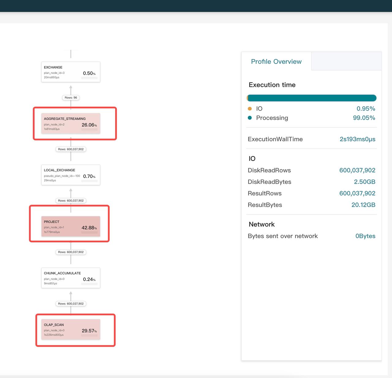
Identify bottlenecks

The larger the proportion of time taken by an operator, the darker color its card becomes. This helps you easily identify bottlenecks of the query.

Check whether data is skewed

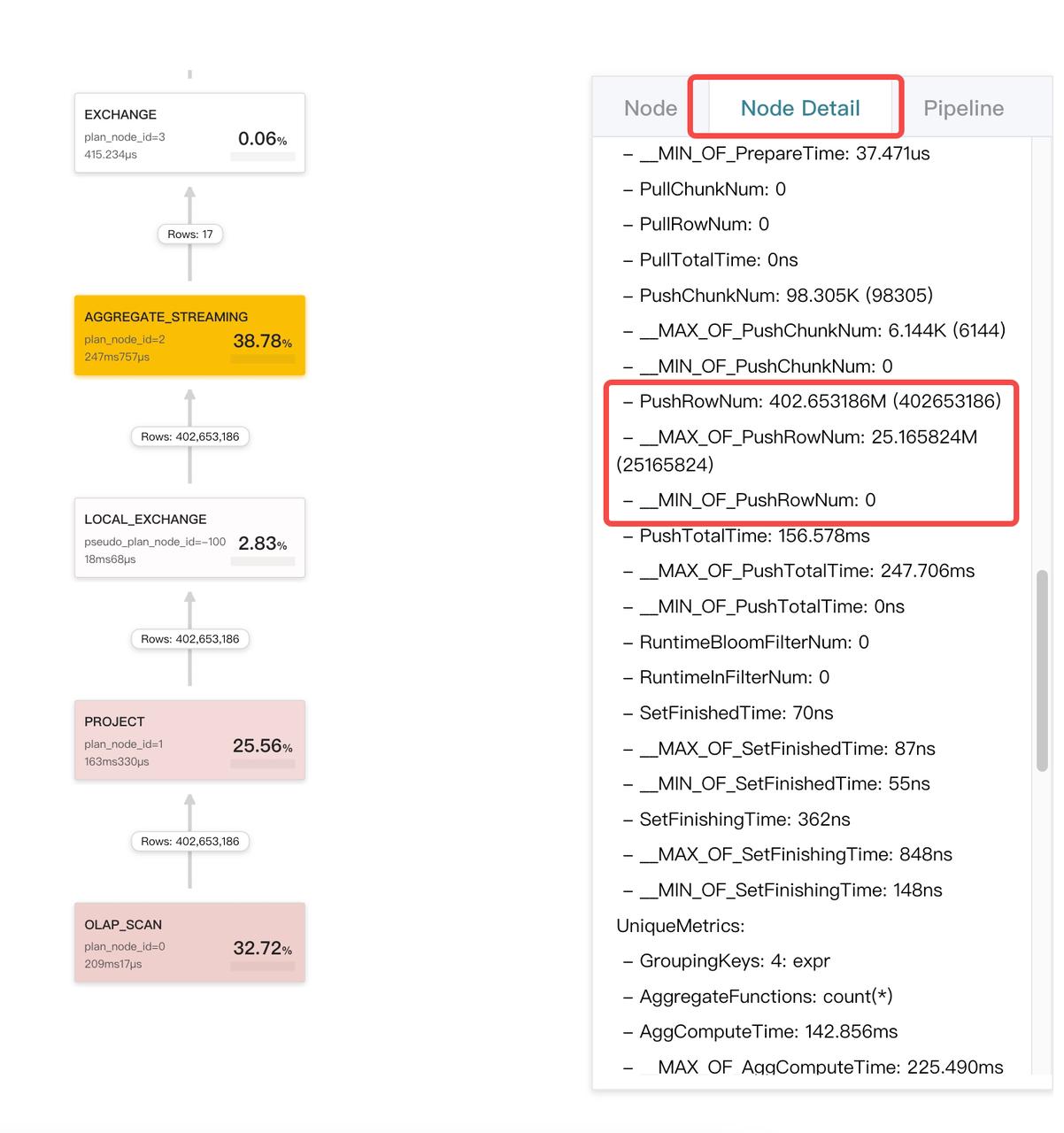
Click the card of the operator that takes a large proportion of time, and check its MaxTime and MinTime. A noticeable difference between MaxTime and MinTime usually indicates data is skewed.

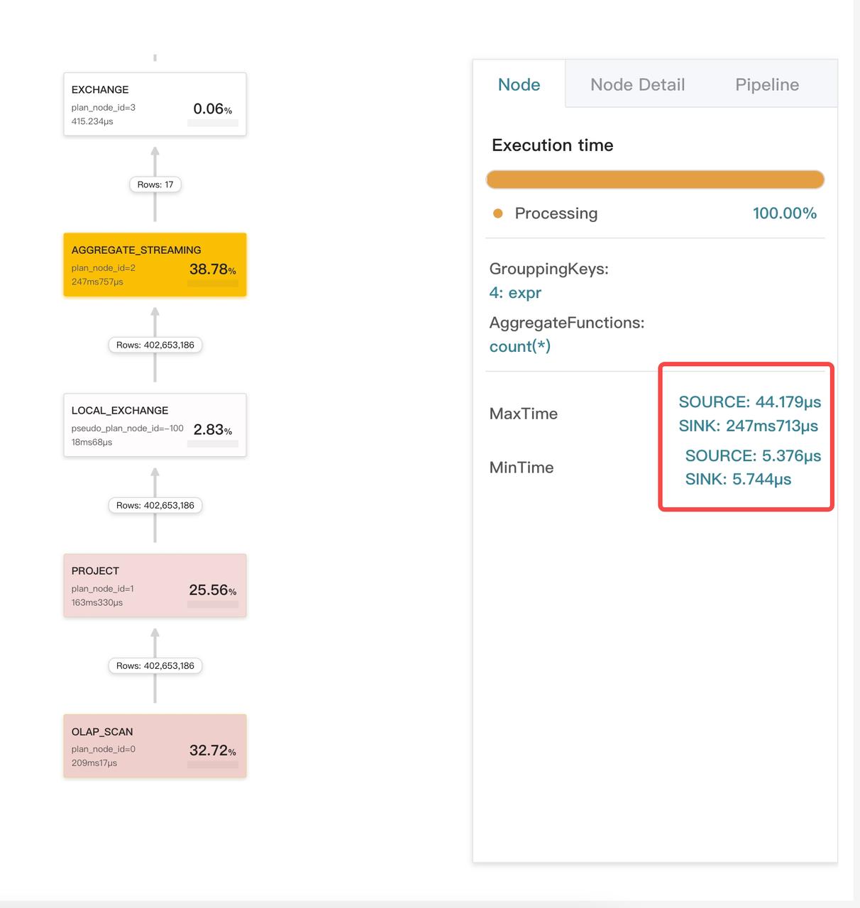
Then, click the Node Detail tab, and check if any metric shows an exception. In this example, the metric PushRowNum of the Aggregate operator shows data skew.

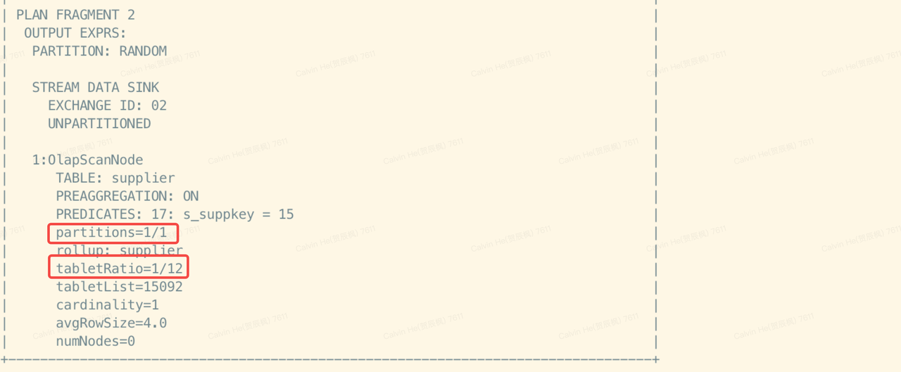
Check whether the partitioning or bucketing strategy takes effect

You can check whether the partitioning or bucketing strategy takes effect by viewing the corresponding query plan using EXPLAIN <sql_statement>.

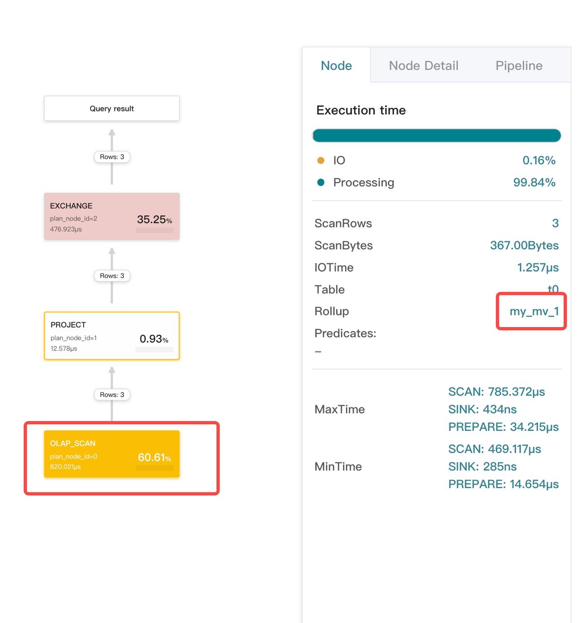
Check whether the correct materialized view is used

Click the corresponding Scan operator and check the Rollup field on the Node Detail tab.

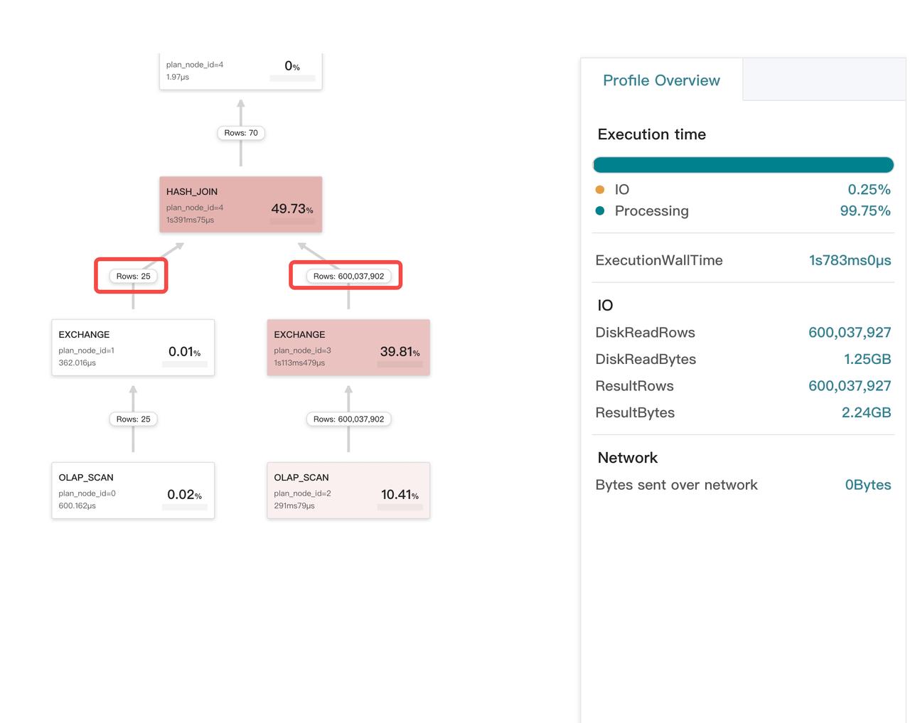
Check whether the JOIN plan is proper for left and right tables

Usually, StarRocks selects the smaller table as the right table of Join. An exception occurs if the query profile shows otherwise.

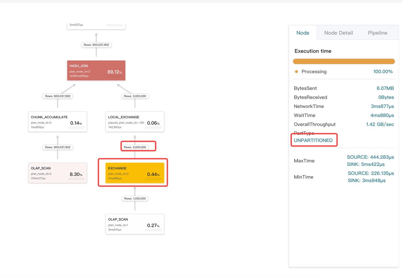
Check whether the distribution type of JOIN is correct

Exchange operators are classified into three types in accordance with the data distribution type:

• UNPARTITIONED: Broadcast. Data is made into several copies and distributed to multiple BEs.
• RANDOM: Round robin.
• HASH_PARTITIONED and BUCKET_SHUFFLE_HASH_PARTITIONED: Shuffle. The difference between HASH_PARTITIONED and BUCKET_SHUFFLE_HASH_PARTITIONED lies in the hash functions used to calculate the hash code.

For Inner Join, the right table can be the HASH_PARTITIONED and BUCKET_SHUFFLE_HASH_PARTITIONED type or UNPARTITIONED type. Usually, UNPARTITIONED type is adopted only when there are less than 100K rows in the right table.

In the following example, the type of the Exchange operator is Broadcast, but the size of data transmitted by the operator greatly exceeds the threshold.

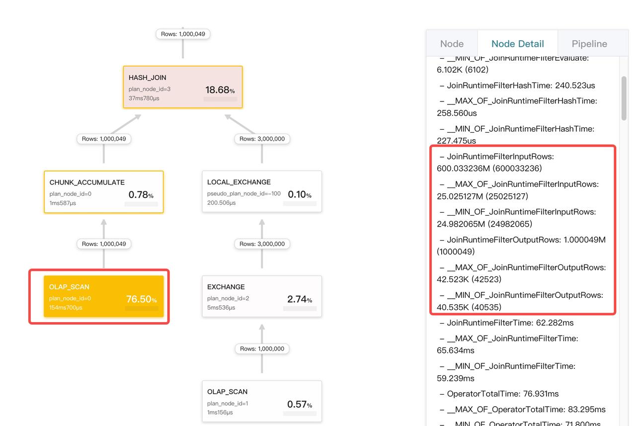
Check whether JoinRuntimeFilter takes effect

When the right child of Join is building a hash table, it creates a runtime filter. This runtime filter is sent to the left child tree, and is pushed down to the Scan operator if it is possible. You can check JoinRuntimeFilter-related metrics on the Node Detail tab of the Scan operator.

FAQ

Why is the time cost of the Exchange operator abnormal?

The time cost of an Exchange operator consists of two parts: CPU time and network time. Network time relies on the system clock. Network time is calculated as follows:

1. The sender records a send_timestamp before calling the bRPC interface to send the package.
2. The receiver records a receive_timestamp after receiving the package from the bRPC interface (post-receiving processing time excluded).
3. After the processing is complete, the receiver sends a response and calculates the network latency. The package transmission latency is equivalent to receive_timestamp - send_timestamp.

If system clocks across machines are inconsistent, the time cost of the Exchange operator hits an exception.

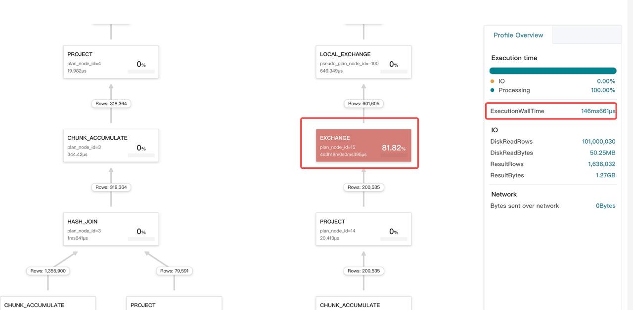
Why is the total time cost of all operators significantly less than the query execution time?

Possible cause: In high-concurrency scenarios, some pipeline drivers, despite being schedulable, may not be processed in time because they are queued. The waiting time is not recorded in operators' metrics, but in PendingTime, ScheduleTime, and IOTaskWaitTime.

Example:

From the profile, we can see that ExecutionWallTime is about 55 ms. However, the total time cost of all operators is less than 10 ms, which is significantly less than ExecutionWallTime.